Formula to calculate difference in rows between the current row and the first row above whose value matches a condition

Question

I can't come up with a combination of functions in Google Sheets that would return the row offset of a cell from another in the same column that matches a given rule.

In the image below is an example using an invented function I named "FIRST_VALUE" to illustrate what I mean:

1. FIRST_VALUE takes two inputs:
   1. A row number:
      ROW() is used in the example, the current row 61
   2. A rule:
      In the example it is ">655"
2. My invented function FIRST_VALUE would return 5 because the value 655,79 is the first value in a row above row 61 that is greater than 655 and it is found in row 56 which is 5 rows above.

I have tried combinations of MATCH, LOOKUP, etc., but none have worked.

This question has also been posted on the Google community help forum: Special function in Google Sheet

Answer 1

You can get that with query(), like this:

=query( 
  sort( { row(A51) - row(A$2:A51) + 1, A$2:A51 }, row(A$2:A51), false ),  
  "select Col1 where Col2 > 655 limit 1",
  0 
)

Answer 2

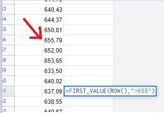
NB: OP is in locale where comma is the decimal separator: $1,00 instead of $1.00. This affects some formula syntax. North American locale syntax shown below each formula followed by // NA.

---

It is unfortunate that you used an invented function to illustrate your problem as it makes it easy to misinterpret the question as being about a Sheets custom function rather than a formula.

There are a few approaches to determine the row difference between the current row and the first one above that also matches a condition.

FILTER w/ MAX

=ROW()-MAX(FILTER(ROW(A:A); ROW(A:A)<ROW(); A:A>655))
=ROW()-MAX(FILTER(ROW(A:A), ROW(A:A)<ROW(), A:A>655))  // NA

	A	B
1	640,43
2	644,37
3	650,81
4	655,79
5	652,00
6	653,65
7	633,50
8	640,02
9	637,09	5 = ROW()-MAX(FILTER(ROW(A:A); ROW(A:A)<ROW(); A:A>655))
10	638,55

=9-FILTER(
   { 1; 2; 3; 4; 5; 6; 7; 8; 9; 10 };
   { 1; 2; 3; 4; 5; 6; 7; 8; 9; 10 } < 8;
   { 640,43; 644,37; 650,81; 655,79; 652,00;
     653,65; 633,50; 640,02; 637,09; 638,55 } > 655))

=9-FILTER(
   { 1; 2; 3; 4; 5; 6; 7; 8; 9; 10 };
   { T; T; T; T; T; T; T; F; F; F  };
   { F; F; F; T; F; F; F; F; F; F  }))

=9-FILTER(
   { 1; 2; 3; 4; 5; 6; 7; 8; 9; 10 };
   { F; F; F; T; F; F; F; F; F; F  }))

=9-4

=5
     

1. FILTER is applied to ROW(A:A) to return all the row numbers from Column A that match both of the following conditions:
   1. The row number is less that the current row's number:

      ROW(A:A)<ROW()
      

   2. The cell's value is greater than 655:

      A:A>655
      

2. The MAX row number returned by the FILTER is the matching row that is closest to but above the current row, which is then subtracted from the current row for the final result.

FILTER w/ MIN

=MIN(FILTER(ROW()-ROW(A:A); ROW(A:A)<ROW(); A:A>655))
=MIN(FILTER(ROW()-ROW(A:A), ROW(A:A)<ROW(), A:A>655))  // NA

Similar to MAX version but subtraction is now moved inside the FILTER function.

SORTN

=SORTN(IF((ROW()-ROW(A:A)>0) * A:A>655; ROW()-ROW(A:A);))
=SORTN(IF((ROW()-ROW(A:A)>0) * A:A>655, ROW()-ROW(A:A),))  // NA

1. SORTN is an array function like FILTER so the IF function inside it is applied to each row in column A.
2. The conditions are multiplied together and return 1 (true) if both are true or 0 (false) if at least one is false.
3. IF's value_if_true is the subtraction of matching row numbers from the current row number.
4. The default SORTN arguments (sort column=1, sort order=asc., max results=1, allow dupes=0) are perfect so they are simply omitted and the result of the formula is the MIN of valid ROW()-ROW(A:A) values.

XMATCH

This one is the shortest, but may not be appropriate depending on the use case. It matches based on first value equal-to or greater-than (not just greater-than) so you will need to add 0,01 onto your search string or if higher precision is required smaller values like 10^-5 (0,00001).

=ROW()-XMATCH(655,01; OFFSET(A:A;;;ROW());1;-1)
=ROW()-XMATCH(655.01, OFFSET(A:A,,,ROW()),1,-1)  // NA